video
Excel: CELL REFERENCE Function
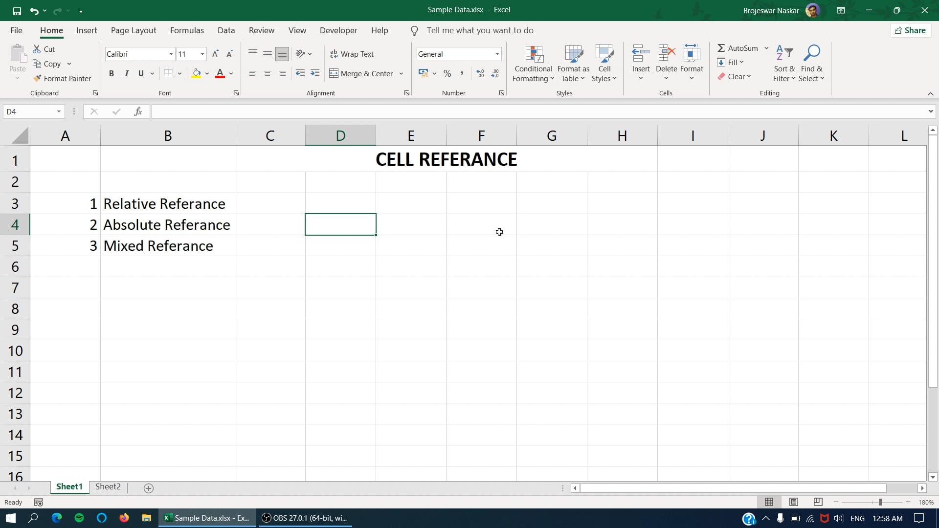
CELL REFERENCE refers to a cell or a range of cells on a worksheet and can be used in a formula. There are three kinds of cell references.
All of us can agree to the fact that Microsoft Excel is the best spreadsheet application that allows users to organize, analyze, and manipulate data in a variety of ways. Its wide range of features help in tasks such as budgeting, financial analysis, data visualization, and more. Additionally, its versatility and ease of use make it a popular tool for both personal and professional use.
Though there are a variety of Excel functions that are commonly used, this page specifically focuses on the Lookup and reference functions in Excel that are used to find specific information in a table or range of data.
The most commonly used lookup function is VLOOKUP (vertical lookup), which searches for a value in the leftmost column of a table and returns a corresponding value in a specified column. Reference functions, such as INDEX and MATCH, can also be used to find specific information in a table. The INDEX function returns a value or the reference to a value from within a table or range, while the MATCH function returns the position of a specified value in a range of cells.
If you are interested to know more about other Lookup and Reference Functions in Excel like OFFSET, HLOOKUP, CELL and INFO, then continue reading!
In Excel, a cell reference refers to the location of a cell in a worksheet. Cell references are used in formulas and functions to refer to the contents or value of a specific cell or range of cells. For example, if the value of cell A1 is 5 and the value of cell B1 is 3, you could use the formula "=A1+B1" in cell C1 to add the values of cells A1 and B1 together and display the result (8) in cell C1. Cell references can also be used to create links between cells, so that if the value in one cell changes, the value in another cell will update automatically.
VLookup (Vertical Lookup) and HLookup (Horizontal Lookup) are functions in Excel that allow you to search for a specific value in a table and return a corresponding value from a specified column.
VLookup searches for a value in the leftmost column of a table, and then returns a value from a specified column to the right. The function has the following syntax:
=VLOOKUP(lookup_value, table_array, col_index_num, [range_lookup])
On the other hand, HLookup (horizontal Lookup) searches for a value in the top row of a table, and then returns a value from a specified row below. The function has the following syntax:
=HLOOKUP(lookup_value, table_array, row_index_num, [range_lookup])
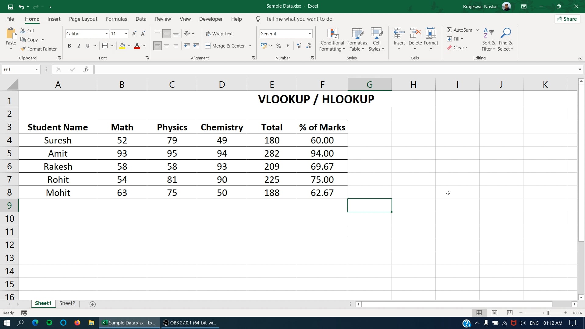
This video tutorial is the first part of a two part series that talks about VLOOKUP & HLOOKUP Function in Excel.
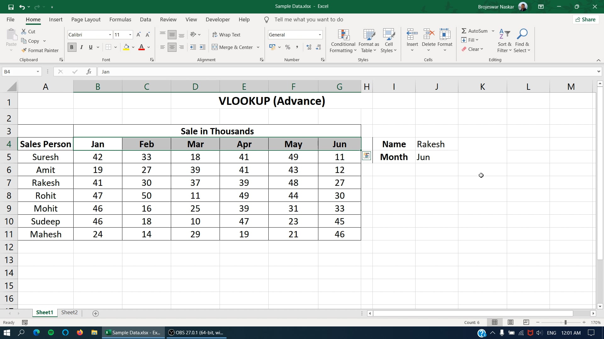
This video tutorial is the first part of a two part series that talks about VLOOKUP & HLOOKUP Function in Excel.
The INDEX function in Excel is a powerful and versatile function that allows you to return a value or the reference to a value from a specific location in a range of cells or array.
The INDEX function can be used in combination with other functions such as MATCH, to create flexible and powerful formulas. For example, you can use the INDEX and MATCH functions together to perform a two-way lookup, where you can look up a value in a table based on both the row and column criteria.
The INDEX function is often used to return a value from a specific location in a large data set, to create dynamic relationships between worksheets and to extract data from a table based on specific conditions.
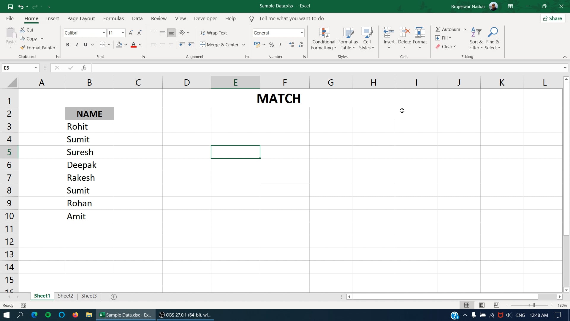
The MATCH function in Excel is a function that returns the position of a value within a range of cells or an array. The function has the following syntax:
=MATCH(lookup_value, lookup_array, [match_type])
The MATCH function returns the position of the first occurrence of the lookup_value within the lookup_array. The position is based on the match_type parameter, if set to 0 it returns the position of the exact match, if set to 1 it returns the position of the next smallest value and if set to -1 it returns the position of the next largest value.
The OFFSET function in Excel is a function that allows you to return a range of cells that is a specified number of rows and columns away from a given reference cell or range. The function has the following syntax:
=OFFSET(reference, rows, cols, [height], [width])
The OFFSET function is useful for creating dynamic ranges that can be used in charts, pivot tables, and other calculations. It allows you to create a range that is based on a specific cell or range, but that can be modified by changing the parameters of the OFFSET function. It's also useful to manipulate data by creating references that change based on the data.
It's worth noting that OFFSET function is volatile, meaning it recalculates with each worksheet change, regardless of whether the precedent data and formulas on which the formula depends have changed, which could impact negatively on the performance of a workbook with many formulas that use the OFFSET function.
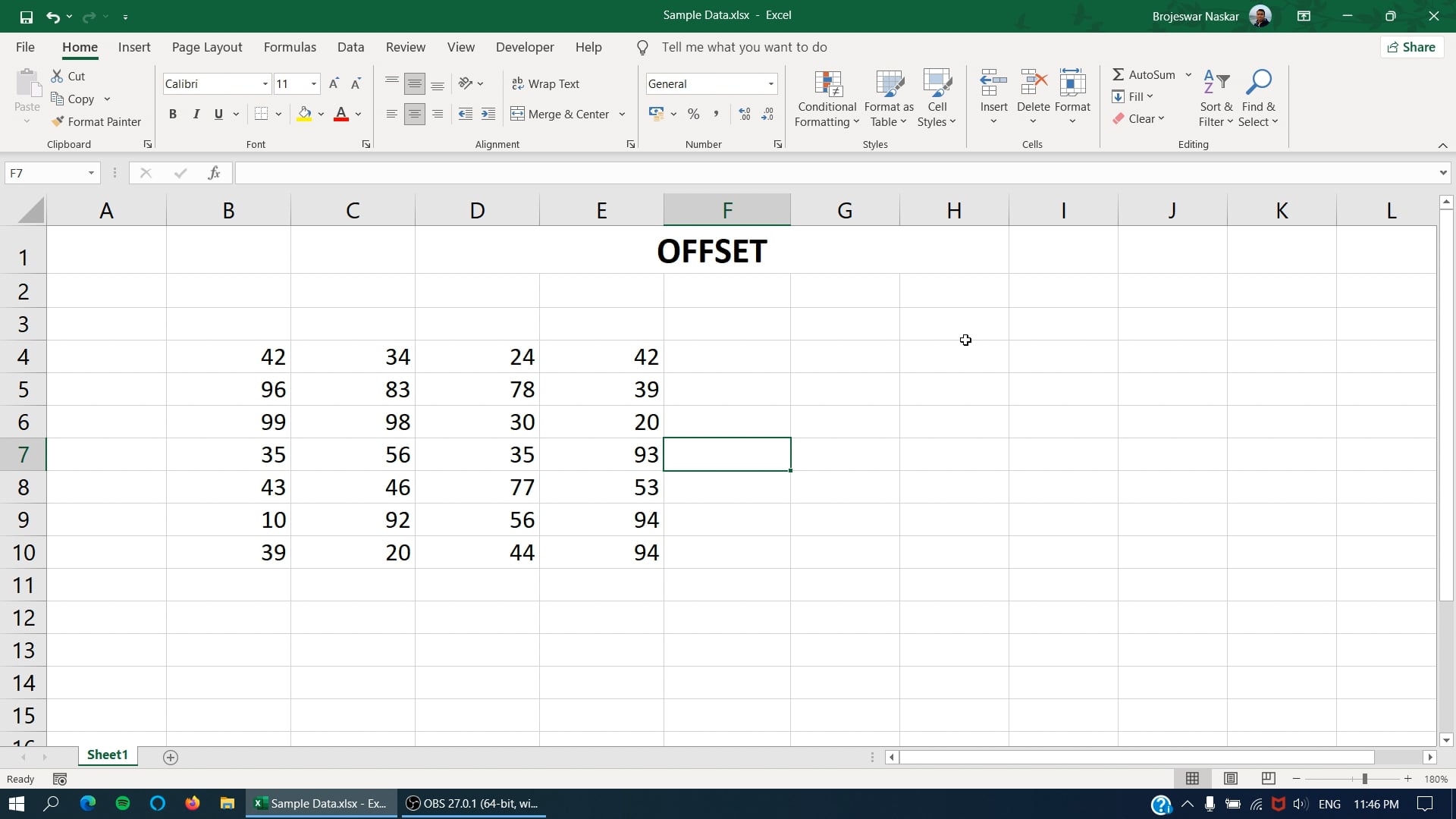
OFFSET returns a reference to a range constructed with five inputs: Starting point, Row offset, Column offset, Height in rows, Width in columns.
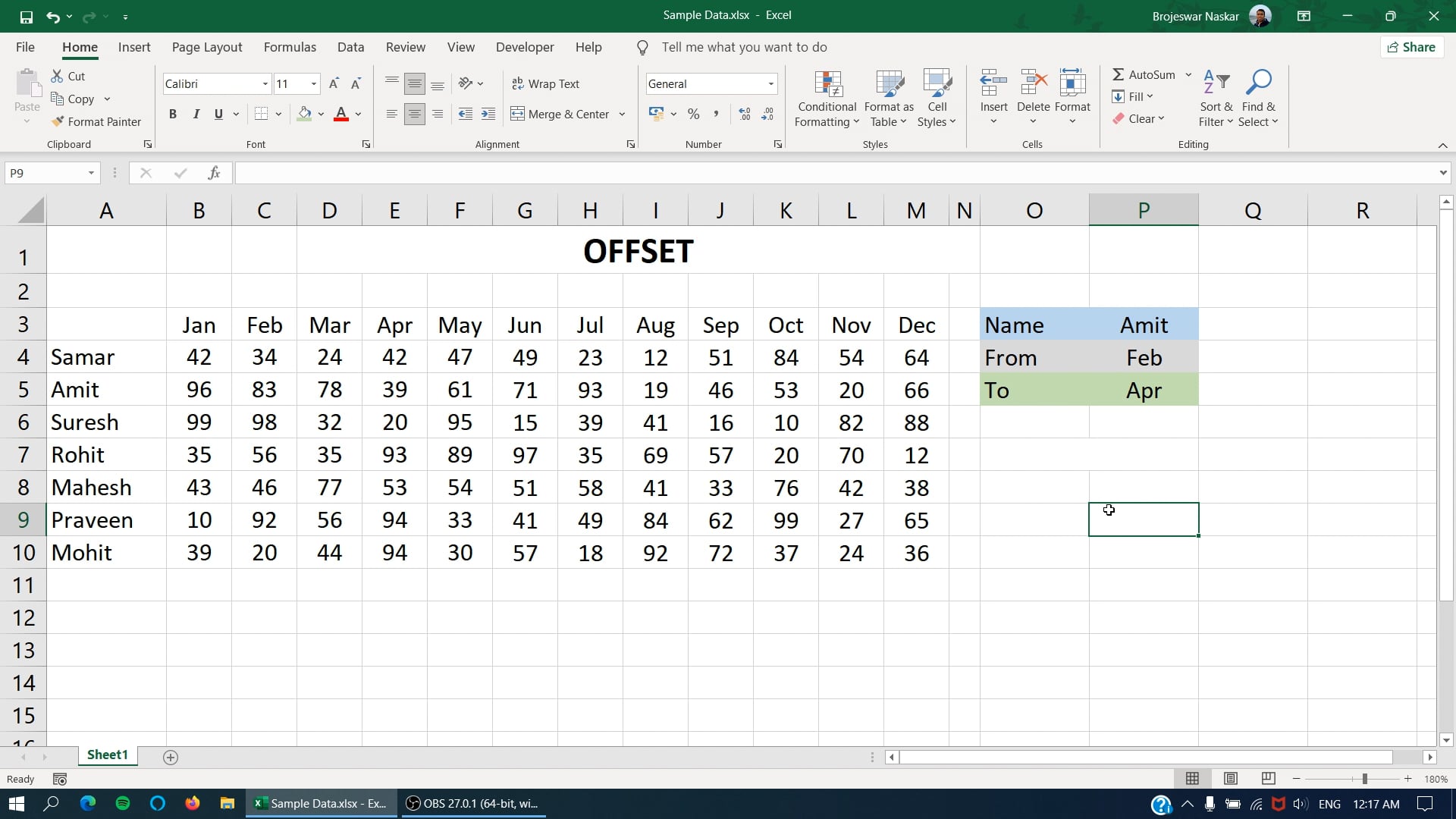
OFFSET returns a reference to a range constructed with five inputs: Starting point, Row offset, Column offset, Height in rows, Width in columns.
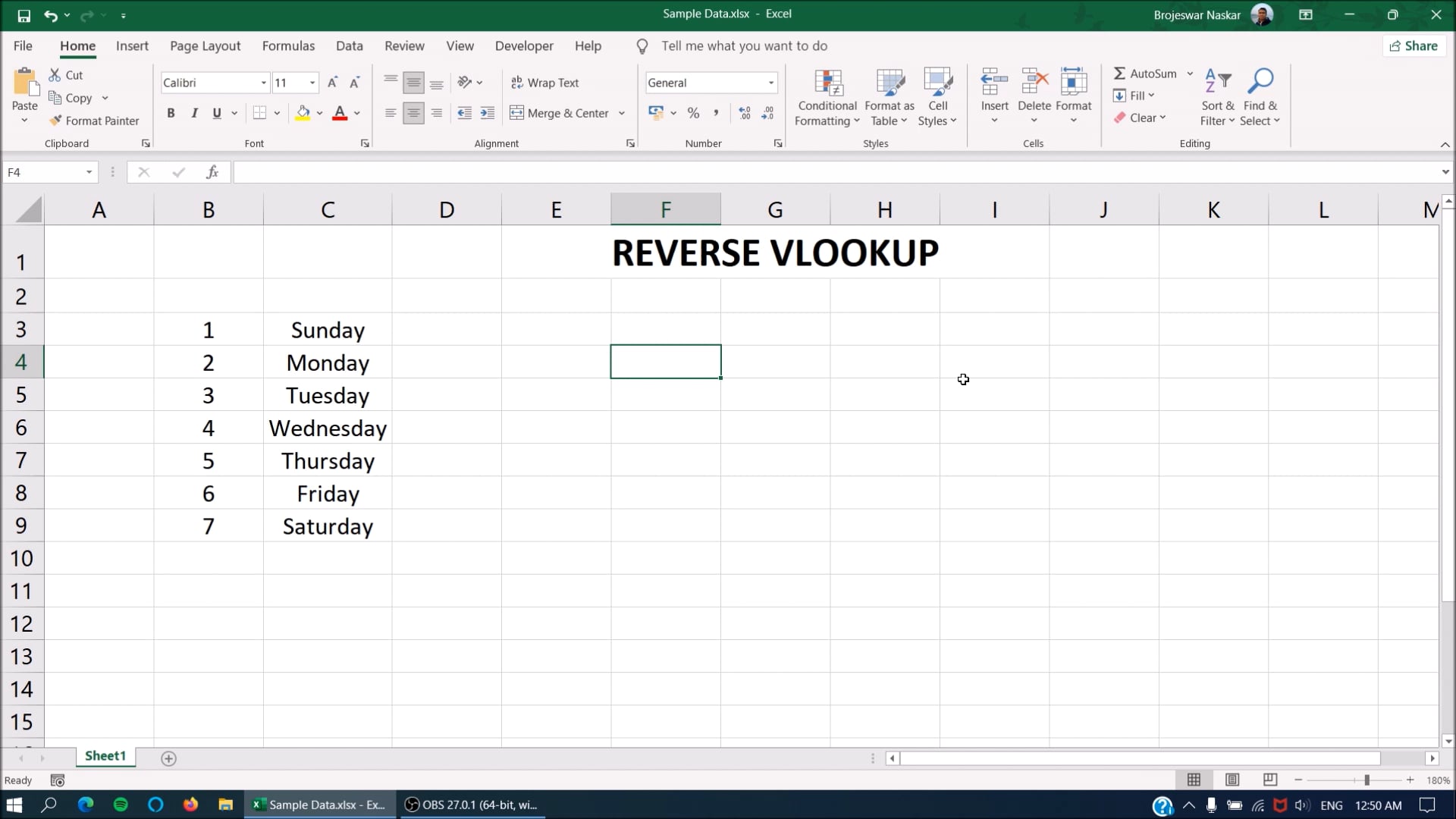
"Reverse Lookup" in Excel refers to the process of finding a value based on a corresponding value in a different column or row. It is the opposite of a traditional lookup where you find a value based on a known value in the same column or row.
There are a few ways to perform a reverse lookup in Excel:
It's worth noting that these methods are not always the most efficient or accurate, and in some cases, it might be necessary to reorganize the data in a way that makes reverse lookup simpler.
CELL: The CELL function returns information about a specific cell in a worksheet. The function has the following syntax: =CELL(info_type, reference). "info_type" is the type of information you want to return, such as the cell's address, color, or contents. "reference" is the cell or range of cells you want to return information about.
INFO: The INFO function returns information about the current operating environment or the status of specific system information. The function has the following syntax: =INFO(type_text).
These functions are useful for automating and streamlining various tasks such as creating dynamic formulas, linking worksheets, and working with large data sets.
Transpose in Excel refers to the process of flipping the rows and columns of a range of cells, so that the rows become columns and the columns become rows. This is useful when you want to change the layout of a data set, or when you need to use a data set in a different format.
There are a few ways to transpose data in Excel:
If you are transposing a large data set, it's advisable to check if all the formulas, conditional formatting, and other features are still working correctly after transposing the data.
Each cell has a unique address, which is the combination of its column letter and row number. For example, the cell at the intersection of column A and row 1 would be cell A1.
These concepts are fundamental to understanding how Excel works, and they are used in many different ways in the program, such as referencing cells, creating formulas, and formatting data. They are also the building blocks for many excel functions and features.
The INDIRECT function in Excel is a function that returns a reference to a range of cells.
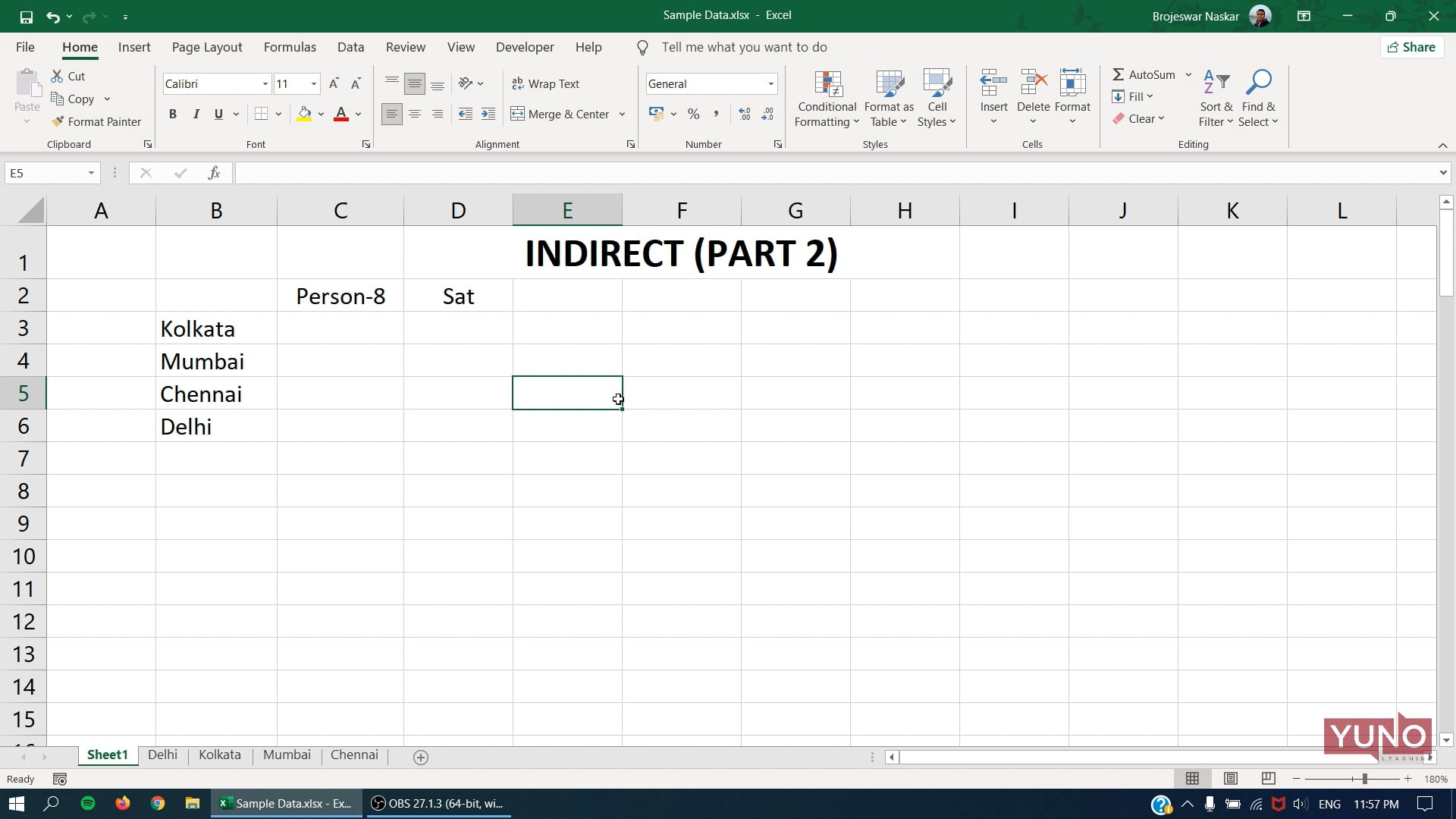
The INDIRECT function is useful for creating dynamic references that can change based on the values in other cells. For example, you can use the INDIRECT function to reference a range of cells that is specified in another cell. You can also use it with other functions such as SUM, COUNTIF, and VLOOKUP to create more dynamic formulas.
It's worth noting that INDIRECT function is volatile, meaning it recalculates with each worksheet change, regardless of whether the precedent data and formulas on which the formula depends have changed, which could impact negatively on the performance of a workbook with many formulas that use the INDIRECT function.
The HYPERLINK function in Excel is a function that creates a hyperlink to a specific location or to a specific file.
You can use the HYPERLINK function to create links to websites, files, and other resources, making it easy for users to access additional information or resources related to the data in the worksheet. The function can be used in a cell, or as part of a formula to generate dynamic links based on the contents of other cells.
You can also create a hyperlink by right-clicking on a cell and selecting "Insert Hyperlink" from the context menu. This will open a dialog box where you can enter the link location and the friendly name.
It's worth noting that when you click on the hyperlink it will open the location (website, file, email) in the default browser or default mail client.
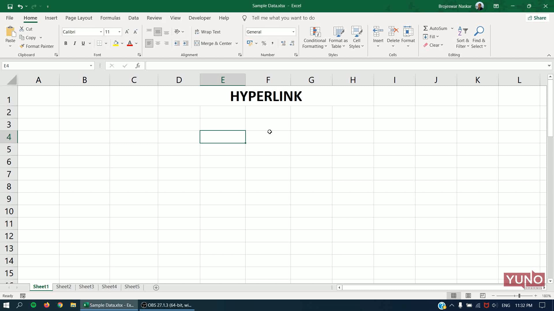
HYPERLINK function returns a hyperlink from a given destination and link text. You can use it to create a clickable hyperlink with a formula.
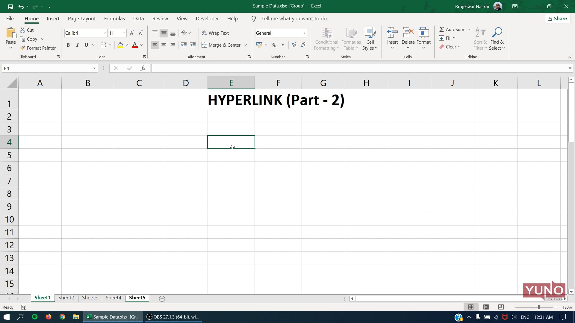
HYPERLINK function returns a hyperlink from a given destination and link text. You can use it to create a clickable hyperlink with a formula.
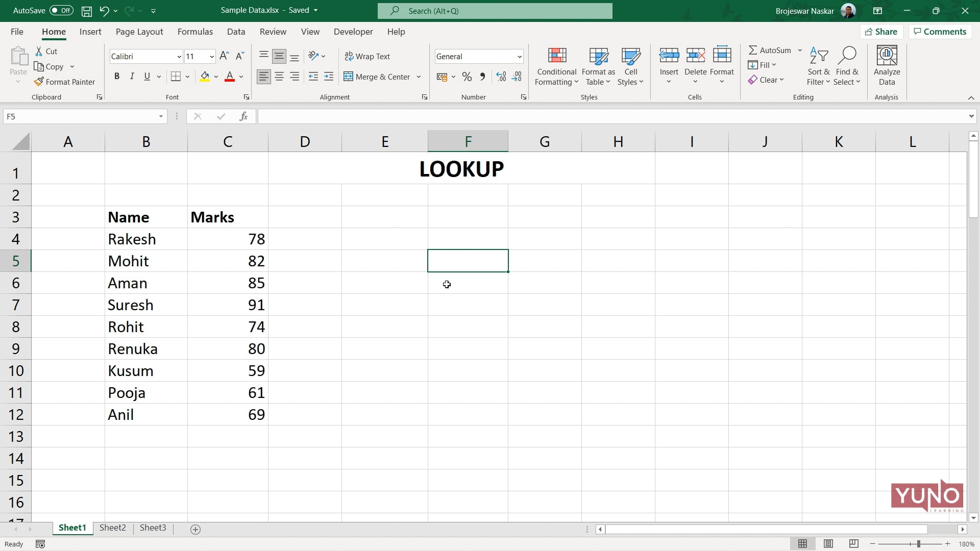
Lookup in Excel refers to the process of finding a specific value within a table or range of cells and returning a corresponding value from another column or row. Excel provides several built-in functions for performing lookups, including: VLOOKUP, HLOOKUP, INDEX and MATCH, etc.
The VLOOKUP (vertical lookup) and HLOOKUP (horizontal lookup) functions in Microsoft Excel are used to find and retrieve data from a specific column or row in a table. VLOOKUP searches for a value in the leftmost column of a table and returns a value from a specified column on the same row. HLOOKUP is similar, but searches for a value in the top row of a table and returns a value from a specified row on the same column. Both functions require at least 3 arguments: the value to search for, the range of cells to search in, and the column or row number to return the value from.
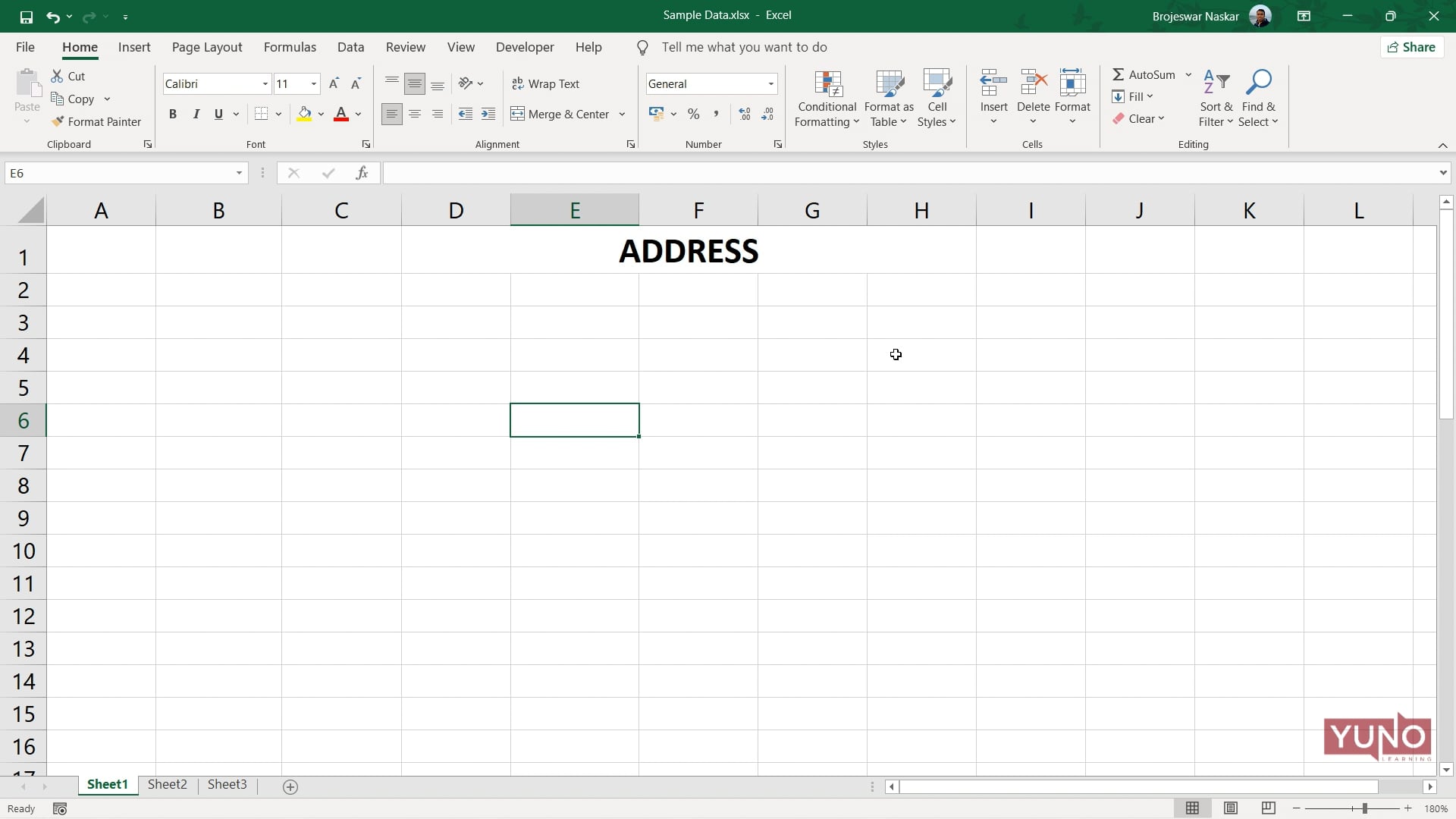
In Microsoft Excel, the ADDRESS function returns a cell address as a text string, based on a specified row and column number. The ADDRESS function has the following syntax:
=ADDRESS(row_num, column_num, [abs_num], [a1], [sheet_text])
For example, the formula =ADDRESS(1,1) will return the address of the cell in the first row and first column of the active sheet, in this case "A1".
Additionally, you can use the INDIRECT function to return a reference to a range of cells, based on the text string of a cell address.
The XLOOKUP function is a new function in Microsoft Excel, which is similar to the VLOOKUP and HLOOKUP functions but more powerful. It allows you to look up and retrieve data from a table based on one or more lookup values, and also support for looking up data to the left.
For example, the formula =XLOOKUP("apple", A2:A5, B2:B5) will return the value in the corresponding cell in column B for the row where the value "apple" is found in column A.
It's important to note that XLOOKUP is only available in Excel versions starting with Office 365 and Excel 2019, If you're using an older version of Excel, you will not be able to use the XLOOKUP function.
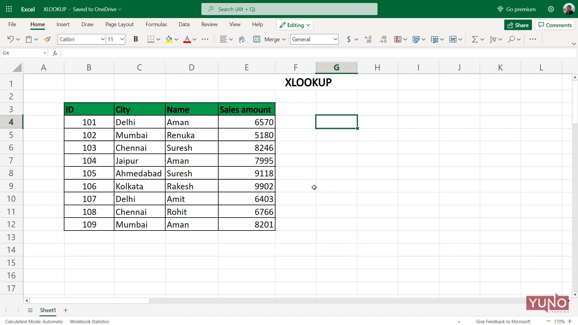
XLOOKUP function is a modern and flexible replacement for older functions like VLOOKUP, HLOOKUP,REVERSE VLOOKUP, LOOKUP, INDEX, MATCH, IFFERROR.
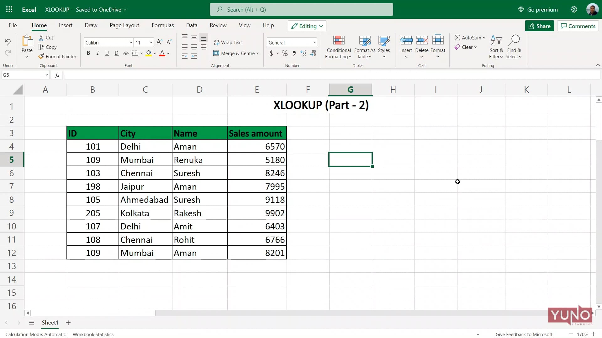
XLOOKUP function is a modern and flexible replacement for older functions like VLOOKUP, HLOOKUP,REVERSE VLOOKUP, LOOKUP, INDEX, MATCH, IFFERROR.
By default, the VLOOKUP function in Microsoft Excel is case-insensitive, meaning it will match values regardless of their capitalization. If you want to make the VLOOKUP case-sensitive, you can use a combination of the VLOOKUP function with the EXACT function.
The EXACT function compares two text strings and returns TRUE if they are exactly the same, including case, and FALSE if they are not.
The formula would be : =VLOOKUP(EXACT(lookup_value,lookup_array), lookup_array, return_array, [match_type])
For example, the formula =VLOOKUP(EXACT("apple",A2:A5), A2:A5, B2:B5) will return the value in the corresponding cell in column B for the row where the value "apple" is found in column A, with case-sensitive.
It's important to note that the EXACT function is case-sensitive, so you will need to make sure that the lookup_value and the values in the lookup_array are entered with the same case for this method to work correctly.
To learn more about advanced excel topics, login to www.yunolearning.com. We also offer courses in Spoken English, Business Writing and IELTS preparation. Send us your inquiries at maya@yunolearning.com or call at +91-8847251466.